
This might be useful for you—alternating the color on a large spreadsheet. Yes, this is easier to do in Microsoft Excel, but with this trick you too can do this in Google Sheets!
The trick is in something called “conditional format rules”, which I’ll explain now.
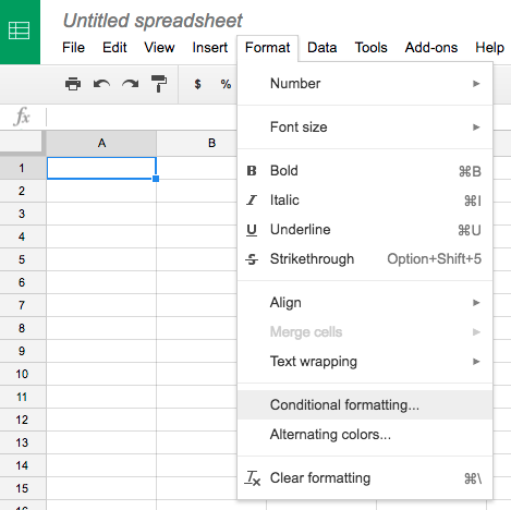 I created a new document but you can be in one you’ve already made if you want. From here I went to the Format menu and then selected Conditional formatting… option.
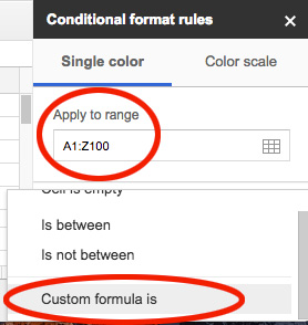 From here, select the range which you will need to work on. In this example I’ve typed in “A1:Z100” (to get a very large range for future data) but if you already know your specific range, then just go with that.
After you’ve selected your range, click on Custom formula is which will bring you to the next step.
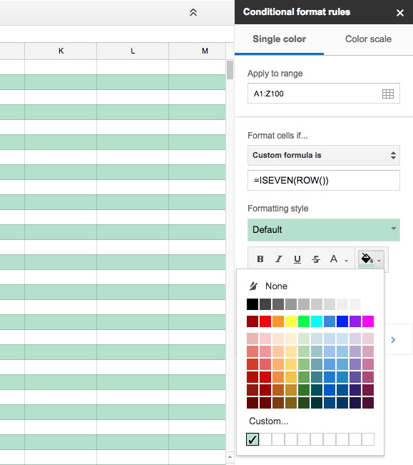
This is going to sound strange, and we don’t expect you to memorize this… but here is the following formula:
=ISEVEN(ROW())
Once you put this in and hit return or enter, you’ll see the change immediately.
Want to enter another set of alternative rows? Click on Add another rule and instead of the previous formula, insert this particular formula. As the second pink arrow illustrates, you can easily change these colors.

=ISODD(ROW())
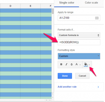
One last note. If you want to do this with columns, change the formula from “(ROW())” to “(COLUMN())”
You must be logged in to post a comment.